Spreadsheets: Conditional Formatting

Conditional formatting is something I only got into recently. I love when my spreadsheets do all kinds of things automatically, especially giving me statistics and pulling certain data from a big sheet. So naturally, because I also like my spreadsheets to look nice, I looked into conditional formatting. The basic usage is pretty simple, but if you want to take it a step further, you need some formulas, so I thought I’ll share how it’s done.

Basic conditions:

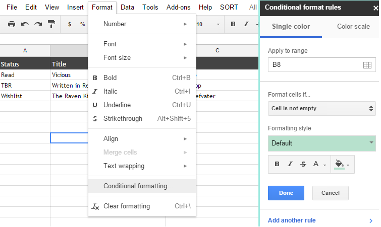
Applying conditional formatting is pretty easy. You can open the editor via the menu and already get a wide variety of options. You just have to define a range and choose a condition and the format.

Some examples of what you can do:

• Format cells with values equal/greater/less than a given value
• Format cells with dates equal/before/after a given date
• Format cells with text equal/containing/starting/ending with a given text
• …

For me, these options are too limited and they can’t do what I want to do. And the format is only applied to the cell that fits the condition. If you want to apply the formatting to a whole row for example, you have to use the last option “Custom formula is…”.

Advanced conditions:

When you use a custom formula, the range now also indicates what range you want the format to be applied to. For formatting to be applied to a whole row, you also have to use the $ notation in the formula. For example range D:D becomes $D:$D and range D2:D5 becomes $D$2:$D$5.

Defining a formula is actually pretty easy. Just think about what you want, define the range for that and put it into an equation. 

Some examples:

• you want to format all rows of books that are marked as Wishlist.
  -> If Status = “Wishlist” then apply format 
  The status is in column A
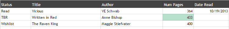
  Formula: =$A:$A=”Wishlist”
• you want to format the row which has the max value of number of pages
  -> If Num Pages = the max value of all numbers then apply format
  The number of pages are in column D and you get the max value with the formula max(range)
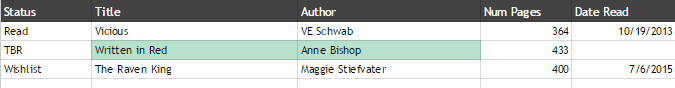
  Formula: =$D:$D=max($D:$D)
• you want to format all rows of books you read in 2015
  -> If Year of Date Read = 2015, then apply format
  The date is in column E, you get the year of a date with the formula Year(date)
  Formula: =YEAR($E:$E)=2015 OR =YEAR($E:$E)=YEAR(TODAY()) to use the current year
• you want to format all rows with page numbers bigger than the value given in cell G1
  -> If Num Pages > G1 then apply format
  Formula: =$D:$D>$G$1
• you want to format every second row (= the rows with even numbers)
  Formula: =ISEVEN(ROW())

One formula, different ranges

Here is just one examples that shows that you can choose any range you want to apply the format to. It doesn’t depend on the range you use for the condition.

Range: D:D
Formula: =$D:$D=max($D:$D)

Range: B:C
Formula: =$D:$D=max($D:$D)

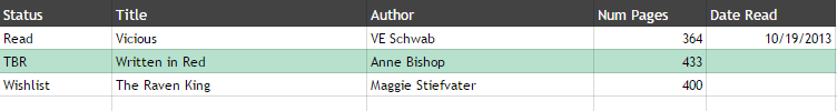
Range: A:E
Formula: =$D:$D=max($D:$D)

Feel free to ask questions in the comments.

For more tutorials see this page.